Monte Carlo Simulation – Deep Value Ideas

Portfolio optimization is of central importance to the field of quantitative finance. Under the assumption that returns follow a multivariate normal distribution with known mean and variance, mean-variance optimization, developed by Markowitz (1952), is mathematically the optimal procedure to maximize the risk-adjusted return. However, it has been shown, e.g., by DeMiguel, Garlappi, and Uppal (2007), that out-of-sample performance of optimized portfolios is worse than that of naively constructed ones. The question is why? Do the results break down if the normality assumption is violated? I will show Monte Carlo evidence under heavy tailed distributions that suggest the cause for this strange phenomenon to be a different one.

The actual problem is that, in practice, mean and variance are not known but need to be estimated. Naturally, the sample moments are estimated with some amount of error. Unfortunately, the solution, i.e., the optimal weight vector, to the optimization problem is very sensitive to these estimation errors. The resulting instability of the solution tends to increase with the number of assets in the universe.

To get an intuition why this would happen, imagine $N$ uncorrelated assets. Hence, the corresponding (unknown) covariance matrix has only zeros off its diagonal. It is, however, very unlikely that a sample covariance matrix will estimate all off-diagonals to be exactly zero, given a finite sample. You can easily see that the probability that this would happen decreases with $N$ . Now, suppose that the estimated sample covariance for some asset $i$ and some other asset $j$ is some positive number. The optimization algorithm now believes that it can reduce the portfolio risk resulting from longing $i$ by shorting $j$ . We know, however, that this would not be optimal since the true data generating processes of $i$ and $j$ are uncorrelated.

The solution to the instability problem is to prevent the optimization algorithm from considering unrelated assets as related. This can be done in two ways. Either we reduce noise in the covariance matrix or we allow hedging between instruments only in certain cases where we have a prior believe that future returns will indeed be correlated. For example, the latter solution implies that we may be comfortable asserting that two airlines expose the portfolio to similar kinds of risk, e.g., oil price, political risk, regulatory risk, travel demand, terror risk, etc., and by selling one of them short we may hedge out these risks resulting from holding long the other. In contrast, just because the sample covariance for an airline stock and some other, totally unrelated, stock is slightly positive, this does not mean we should sell short a large chunk of that second stock to hedge out the risks of the airline stock, although the mean-variance optimizer would regard both scenarios the same.

For me, the best way to get a deeper understanding of the subject is to simulate sample paths, where I know the data generating process, and to observe the behavior of different optimization techniques. In the following, I will compare mean-variance optimization based on sample moments with the same based on a noise-reduced covariance matrix using principal component analysis (PCA). To demonstrate the other approach, I will introduce a hierarchical optimization algorithm, where I use the fact that stocks usually cluster into industries. As a lower bound benchmark, I show results for naive equal weighting. We will see that, out-of-sample, portfolios based on the sample covariance matrix underperform this benchmark substantially. The PCA and hierarchical methods, however, perform significantly better. These results are robust to heavy tailed noise distributions as evidenced by simulated Generalized Autoregressive Conditional Heteroscedasticity (GARCH) sample paths.

But first, let’s simulate a bunch of stocks belonging to different industries. Each stock is composed of a deterministic trend $\mu$ , a loading on the market related stochastic trend $\beta_{market}$ and a loading on the industry specific stochastic trend $\beta_{industry}$ . For each stock, $\mu$ , $\beta_{market}$ , and $\beta_{industry}$ are sampled from a uniform distribution. In the first simulation, I compare mean-variance optimization with a naive diversification approach where each asset is equally weighted with the sign of the expected return. I assume perfect knowledge of the expected return. Traditionally, the expected return is estimated by the in-sample first moment of the asset return. In my example, this would actually make sense since the mean is a consistent estimator of the deterministic trend. In practice, however, there is probably not a stationary deterministic trend. This is where the alpha model steps in, which is not the topic of this study and thus assumed given.

The return of each stock is thus given by

$R_{i t} = \mu_{i}+\beta_{i 1}f_{1 t}+\beta_{i 2} f_{2 t}+\cdots+\beta_{i k} f_{k t}+\epsilon_{i t} = \mu_{i}+\sum_{\ell=1}^{k} \beta_{i \ell} f_{\ell t}+\epsilon_{i t}$ ,

where

$R_{i t}$ is the return of asset $i$ at time $t$ ,
${f_{\ell t}}$ is the $\ell$ th common factor at time $t$ ,
$\beta_{i \ell}$ is the factor loading or factor beta of asset $i$ with respect to factor $\ell$ ,
$\epsilon_{i t}$ is the asset-specific factor or asset-specific risk,
$i=1, \ldots, N$ ,
$\ell=1, \ldots, k$ .

The $k \times k$ covariance matrix of the factors, $\boldsymbol{f}_{t}=\left[f_{1 t}, f_{2 t}, \ldots, f_{k t}\right]^{\prime}$ , is $\mathrm{Cov}\left(\boldsymbol{f}_{t}\right)=\boldsymbol{\Sigma}_{f}$ . Asset-specific noise is uncorrelated with the factors, i.e., $\mathrm{Cov}\left(f_{\ell t}, \epsilon_{i t}\right)=0$ , for $\ell=1, \ldots, k$ , $i=1, \ldots, N$ , and $\quad t=1, \ldots, T$ . The asset-specific noise is uncorrelated across assets and for each asset it’s serially uncorrelated, i.e.,

${\qquad \boldsymbol{\Sigma}_{\boldsymbol{\epsilon}}=\mathrm{Cov}\left(\boldsymbol{\epsilon}_{t}\right)=\left[\begin{array}{cccc}{\sigma_{\epsilon_{1}}^{2}} & {0} & {\cdots} & {0} \\ {0} & {\sigma_{\epsilon_{2}}^{2}} & {\cdots} & {0} \\ {\vdots} & {\vdots} & {\ddots} & {\vdots} \\ {0} & {0} & {\cdots} & {\sigma_{\epsilon_{N}}^{2}}\end{array}\right]}$ .

The diagonal covariance structure reflects the assumption that all correlation between assets is due to the factors.

Let’s write the factor model as

$\boldsymbol{R}_{t}=\boldsymbol{\alpha}+\boldsymbol{B} \boldsymbol{f}_{t}+\boldsymbol{\epsilon}_{t}$ ,

where in the $N \times k$ matrix $\boldsymbol{B}$ ,

${\qquad \boldsymbol{B}=\left[\begin{array}{c}{\boldsymbol{\beta}_{1}^{\prime}} \\ {\boldsymbol{\beta}_{2}^{\prime}} \\ {\vdots} \\ {\boldsymbol{\beta}_{N}^{\prime}}\end{array}\right]=\left[\begin{array}{cccc}{\beta_{11}} & {\beta_{12}} & {\cdots} & {\beta_{1 k}} \\ {\beta_{21}} & {\beta_{22}} & {\cdots} & {\beta_{2 k}} \\ {\vdots} & {\vdots} & {\ddots} & {\vdots} \\ {\beta_{N 1}} & {\beta_{N 2}} & {\cdots} & {\beta_{N k}}\end{array}\right]}$ ,

the $\ell$ th column contains the beta coefficients associated with factor $\ell$ . The covariance matrix of the returns $\boldsymbol{R}_{t}=\left[R_{1 t}, R_{2 t}, \ldots, R_{N t}\right]$ implied by the factor model is

$\boldsymbol{\Sigma}=\mathrm{Cov}\left(\boldsymbol{R}_{t}\right)=\boldsymbol{B} \boldsymbol{\Sigma}_{f} \boldsymbol{B}^{\prime}+\boldsymbol{\Sigma}_{\epsilon}$ .

Hence, the variance of the returns of asset $i$ and the covariance of the returns of asset $i$ and $j$ are

$\mathrm{Var}\left(R_{i}\right)=\beta_{i}^{\prime} \boldsymbol{\Sigma}_{f} \beta_{i}+\sigma_{\epsilon_{i}}^{2}$

and

$\mathrm{Cov}\left(R_{i}, R_{j}\right)=\beta_{i}^{\prime} \boldsymbol{\Sigma}_{f} \beta_{j}$ ,

respectively. Since the factors are uncorrelated in this simulation, the covariance matrix simplifies to

$\boldsymbol{\Sigma}=\boldsymbol{B} \boldsymbol{\Sigma}_{f} \boldsymbol{B}^{\prime}+\boldsymbol{\Sigma}_{\epsilon}=\sum_{\ell=1}^{K} \beta_{\ell} \beta_{\ell}^{\prime} e_{f_{\ell}}^{2}+\Sigma_{\epsilon}$ ,

where $\beta_{\ell}$ is the vector of loadings with respect to factor $\ell$ , i.e., the $\ell$ th column of matrix $\boldsymbol{B}$ . Thus the variance of asset $i$ ‘s returns is

$\sigma_{i}^{2}=\sum_{\ell=1}^{k} \beta_{i \ell}^{2} \sigma_{f_{\ell}}^{2}+\sigma_{\epsilon_{i}}^{2}$

and the covariance between the returns of assets $i$ and $j$ is

$\sigma_{i j}=\sum_{\ell=1}^{k} \beta_{i \ell} \beta_{j \ell} \sigma_{f_{\ell}}^{2}$ .

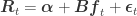
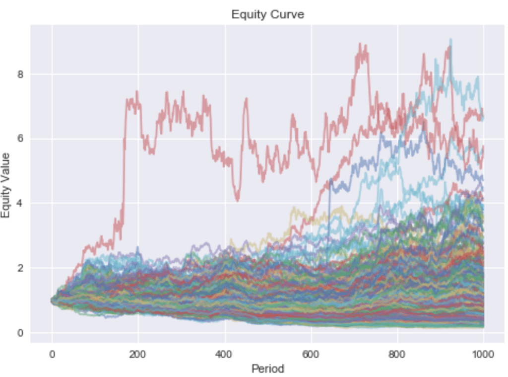
As an example, Figure 1 shows sample paths of 100 stocks belonging to the same industry.

Every stock’s return in this universe is partly driven by the market return (in proportion to its $\beta_{market}$ ) and the industry return (in proportion to its $\beta_{industry}$ ). Hence, one asset can be used to hedge out the factor risks of the other by selling it short. Doing this by mean-variance optimization based on the sample covariance matrix (and known expected return), the resulting portfolio equity under period-wise rebalancing develops as shown in Figure 2.

This very smooth equity curve can be achieved since we can hedge out the systematic factor risk. This makes our bets independent. Independence allows us to reason by the weak law of large numbers that the realized returns will converge in probability to the expected returns. This is only true if short sales are permitted. If we exclude shorting, we can only reduce the asset specific risk while exposing the portfolio to the irreducible systematic risk. The devastating effect this has on our portfolio can be seen by the much more rugged equity curve in Figure 3.

Hierarchical Optimization

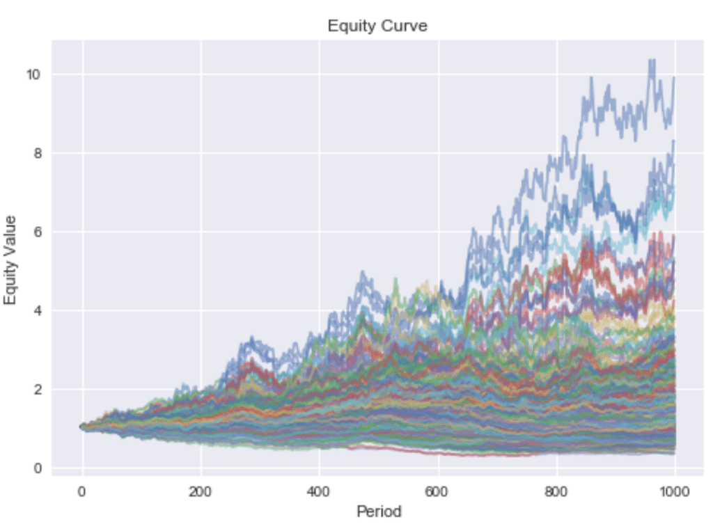
In reality there isn’t just one industry but many. In the following, I will simulate a universe of stocks belonging to nine different industries. The corresponding sample paths are depicted in Figure 4.

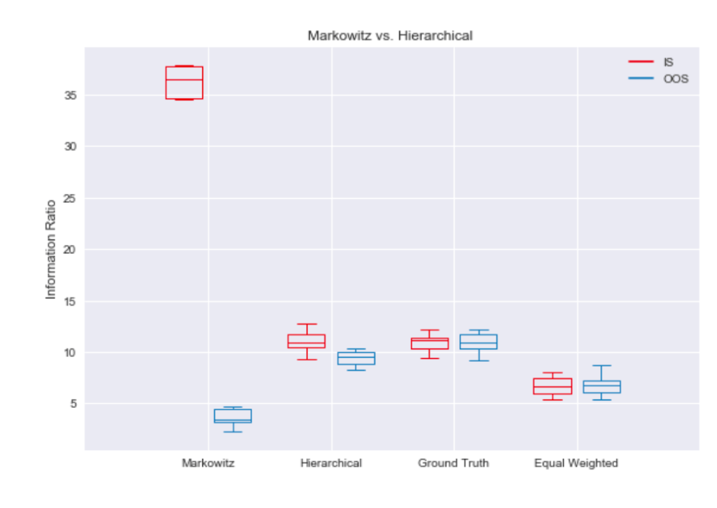
Now, all stocks are still partly driven by the market, but industry returns are uncorrelated. Estimation errors may cause problems if one stock is falsely used as a hedging device for the industry exposure of another stock, and both stocks do not belong to the same industry. The overfit of Markowitz’s method to in-sample data can best be visualized by a boxplot. Figure 5 shows that the in-sample information ratio for the sample covariance optimization is way above the best possible portfolio using ground truth parameters. Unsurprisingly, this overfit hurts the out-of-sample performance, as it can’t even beat simple equal weighting.

If we believe the above characterization of the problem is correct, it seems like a good idea to encode prior knowledge of industry clustering by optimize weights within clusters and then optimize allocation to these clusters. This hierarchical approach results in the in-sample and out-of-sample performance being much closer to the ground truth. Imposing structure, mean-variance optimization now beats equal weighting by a large margin.

Principal Component Analysis

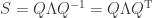
Principal Component Analysis (PCA) allows us to reduce the rank of the covariance matrix. Since the covariance matrix is symmetric positive definite, we can, due to the spectral theorem, decompose the matrix into its real eigenvalues and orthonormal eigenvectors.

$S=Q \Lambda Q^{-1}=Q \Lambda Q^{\mathrm{T}}$ with $Q^{-1}=Q^{\mathrm{T}}$

In the simulation we have exposure to the market and several industries. Thus, it makes sense to reduce the rank to the number of these variables. Plotting the proportion of variance explained by the first $n$ principal components in Figure 6 confirms this hypothesis.

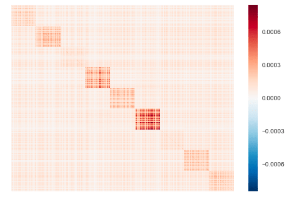
Decomposing the covariance matrix into its eigenvalues and eigenvectors, we can de-noise it by eliminating all eigenvalues below some threshold. Since the sample covariance matrix is positive definite, all its eigenvalues will be positive. Reconstructing a matrix from non-negative eigenvalues will likewise result in a positive semi-definite matrix. We thus don’t have to worry about the resulting matrix not being a proper covariance matrix, which can be a headache with more flexible estimation approaches. A heatmap of the reconstructed covariance matrix from the largest 10 eigenvalues is shown in Figure 7.

This covariance matrix looks very similar to the sample covariance matrix shown in Figure 8, despite having only a rank of 10. We can infer that it captures the important linear relationships between assets with less noise.

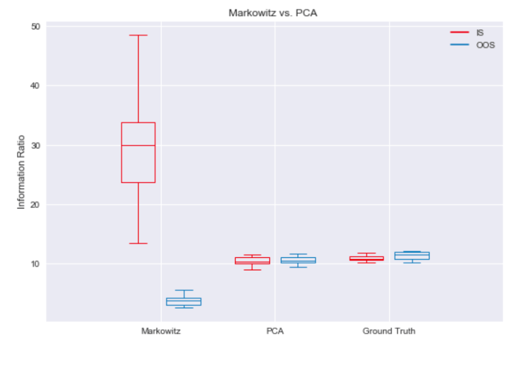
Observing the information ratios depicted in Figure 9, the PCA de-noising method seems capable of restricting factor hedging attempts to reasonable candidates. It beats mean-variance optimization based on the sample covariance matrix in out-of-sample data by a large margin.

Robustness under heavy tailed distributions

Until now, we’ve assumed Gaussian returns. It is a well known fact, though, that real stock return distributions are not Gaussian but heavy tailed. In the following, we will look at simulation results when asset specific noise is modeled by a GARCH process.

Asset specific noise, $\epsilon_{i, t}$ , is now defined by

$\epsilon_{i, t}=\sigma_{i, t} \eta_{t}$ ,

where

$\sigma_{i, t}^{2}=\omega+\sum_{n=1}^{q} \alpha_{n} \epsilon_{i, t-n}^{2}+\sum_{m=1}^{p} \beta_{m} \sigma_{t-m}^{2}$
$\eta_{t} \stackrel{\text {iid}}{\sim}(0,1)$
$\omega>0$
$\alpha_{n} \geq 0$
$\beta_{m} \geq 0$
$m=1, \ldots, p$
$n=1, \ldots, q$

The unconditional variance of asset $i$ ‘s specific noise distribution is

$\mathrm{E}\left(\sigma_{\epsilon_{i, t}}^{2}\right)=\omega+\sum_{n=1}^{q} \alpha_{n} \mathrm{E}\left(\epsilon_{i, t-n}^{2}\right)+\sum_{m=1}^{p} \beta_{m} \mathrm{E}\left(\sigma_{\epsilon_{i, t-m}}^{2}\right) =\omega+\left(\sum_{n=1}^{q} \alpha_{n}+\sum_{m=1}^{p} \beta_{m}\right) \mathrm{E}\left(\sigma_{\epsilon_{i, t}}^{2}\right)$ ,

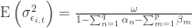
which, when solved for $\mathrm{E}\left(\sigma_{\epsilon_{i, t}}^{2}\right)$ becomes

$\mathrm{E}\left(\sigma_{\epsilon_{i, t}}^{2}\right) = \frac{\omega}{1-\sum_{n=1}^{q} \alpha_{n}-\sum_{m=1}^{p} \beta_{m}}$ .

I use this result to compute the ground truth covariance matrix. Sample paths according to a GARCH(1,1) data generating process are shown in Figure 10.

It’s easy to see that returns are much more extreme than under Gaussian noise. Since Markowitz’s mean-variance optimization tends to over-concentrate and thus expose the portfolio to asset specific risks, which are now heavy tailed, it performs even worse than in the Gaussian case. As shown in Figure 11, the hierarchical method still outperforms equal weighting.

Noise filtering by PCA results in portfolio performances near the ground truth, as can be seen in Figure 12.

Conclusion

To maximize risk-adjusted returns, it is necessary to hedge out systematic risk. How this hedging is done is the subject of portfolio optimization. We’ve seen that it’s important to regularize portfolio optimization, since estimation errors of the covariance matrix would otherwise push out-of-sample performance below that of naive approaches. How to achieve the regularization is a research topic all on its own. We’ve seen two approaches that can be developed far beyond the basics shown here. In addition, correlations between assets tend to be non-stationary. This fact needs to be respected as well. Furthermore, asset returns are driven by multiple factors and business models spread further into sub-clusters within industries. Larger corporations may also belong to multiple clusters. There’s so much more to learn. The code of the simulation, every plot shown here, and all the methods used to compute the portfolio weights is available at https://github.com/jpwoeltjen/OptimizePortfolio.

References

DeMiguel, Victor, Lorenzo Garlappi, and Raman Uppal. “Optimal versus naive diversification: How inefficient is the 1/N portfolio strategy?.” The review of Financial studies 22.5 (2007): 1915-1953.

Markowitz, Harry. “Portfolio selection.” The journal of finance 7.1 (1952): 77-91.