Corporate filings provide a wealth of information and are available for all major publicly traded corporations. Apart from financial statements, most of the information is in textual form. To make them usable in algorithmic trading strategies one has to preprocess them with tools from natural language processing. In the following, I’ll demonstrate a method to construct clusters of stocks based on similarity of documents. In addition, topic modeling by singular value decomposition (SVD) and latent Dirichlet allocation (LDA) of Blei et al. (2003) is used to estimate exposures to risk factors.
Hierarchical Clustering by 10-K Item 1
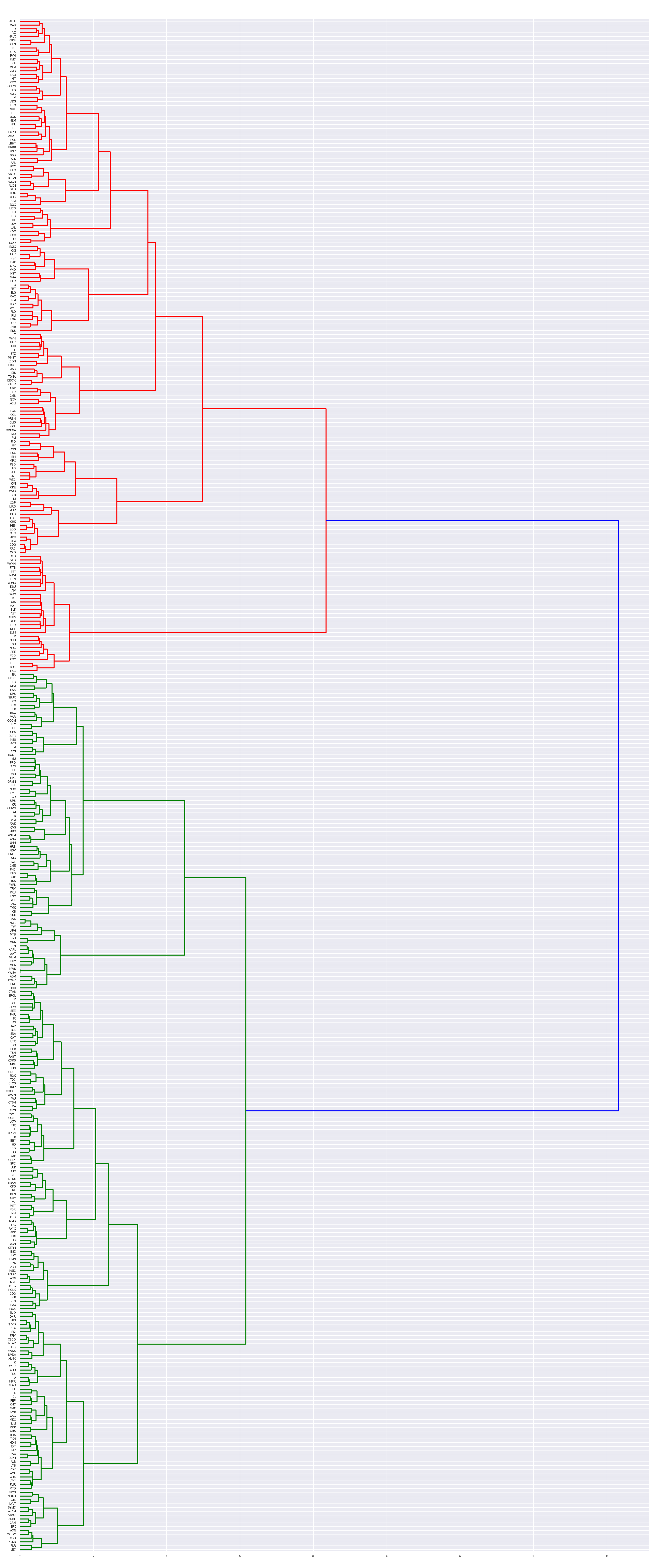
10-K filings of the 500 largest US stocks are downloaded. Certain sections such as Item 1 and Item 1A are extracted based on regex rules. 387 documents for each section remain after filtering. Next, a machine readable term-document matrix is constructed via a tfidf-vectorizer. To cluster stocks according to the business description the cosine similarity matrix of the vectorized Item 1 is fed into a ward clustering algorithm and the resulting linkage matrix is visualized via a dendrogram in Figure 1.
Figure 1
Three main clusters with many sub clusters emerge. The cluster colored in red, for instance, groups banks together.
Topic Modeling of 10-K Item 1
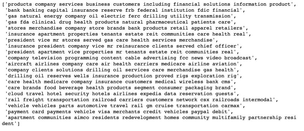
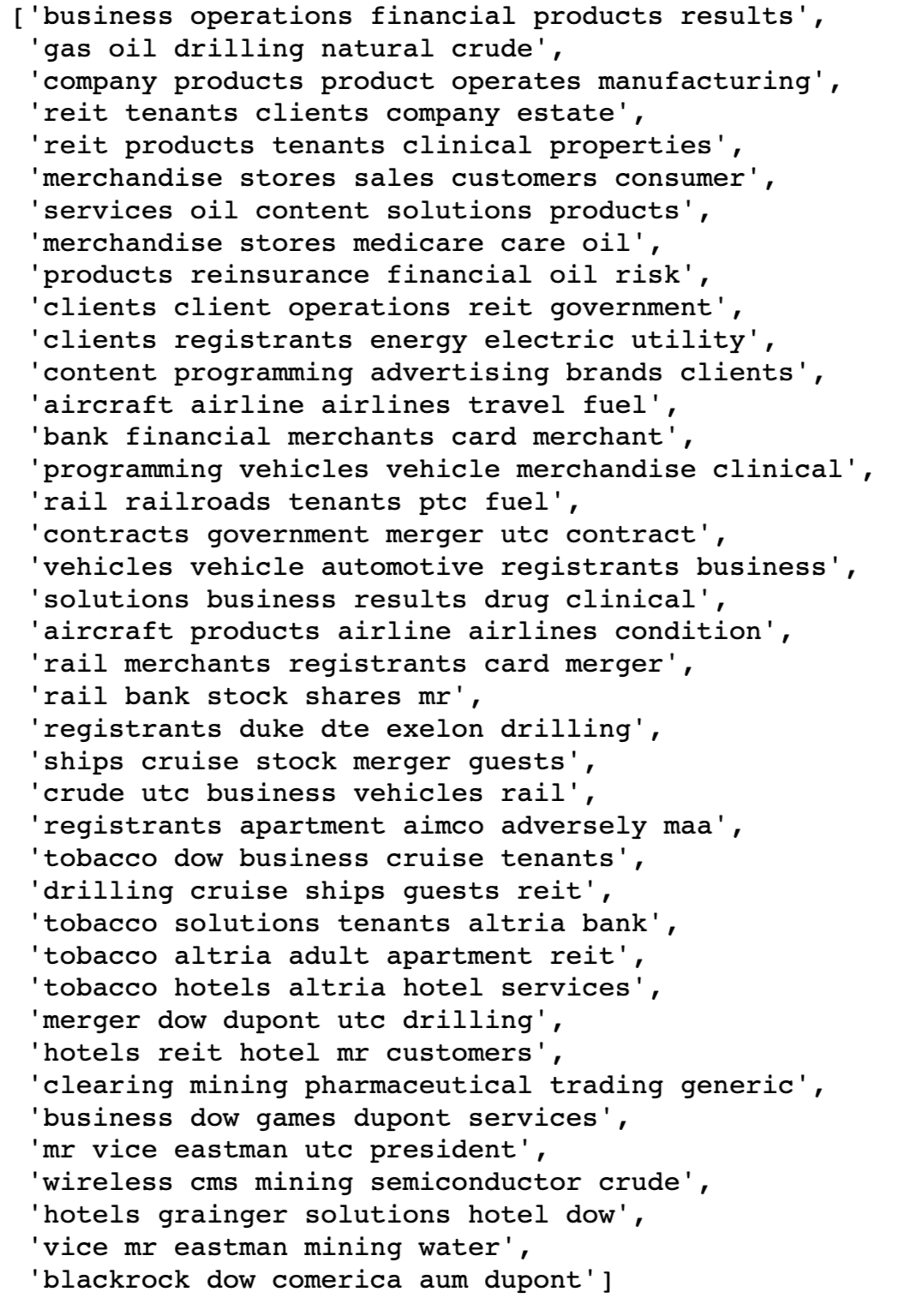
By singular value decomposition (SVD) of the tfidf-vectorized matrix, we can extract the most important topics. Figure 2 displays the 20 most important topics with its respective 10 most common terms. While not perfect — keep in mind we’re only using 387 documents — some clear patterns emerge. For example, the second topic relates to financial institutions, the third topic relates to energy companies, and the fourth topic relates to pharmaceuticals.
Figure 2
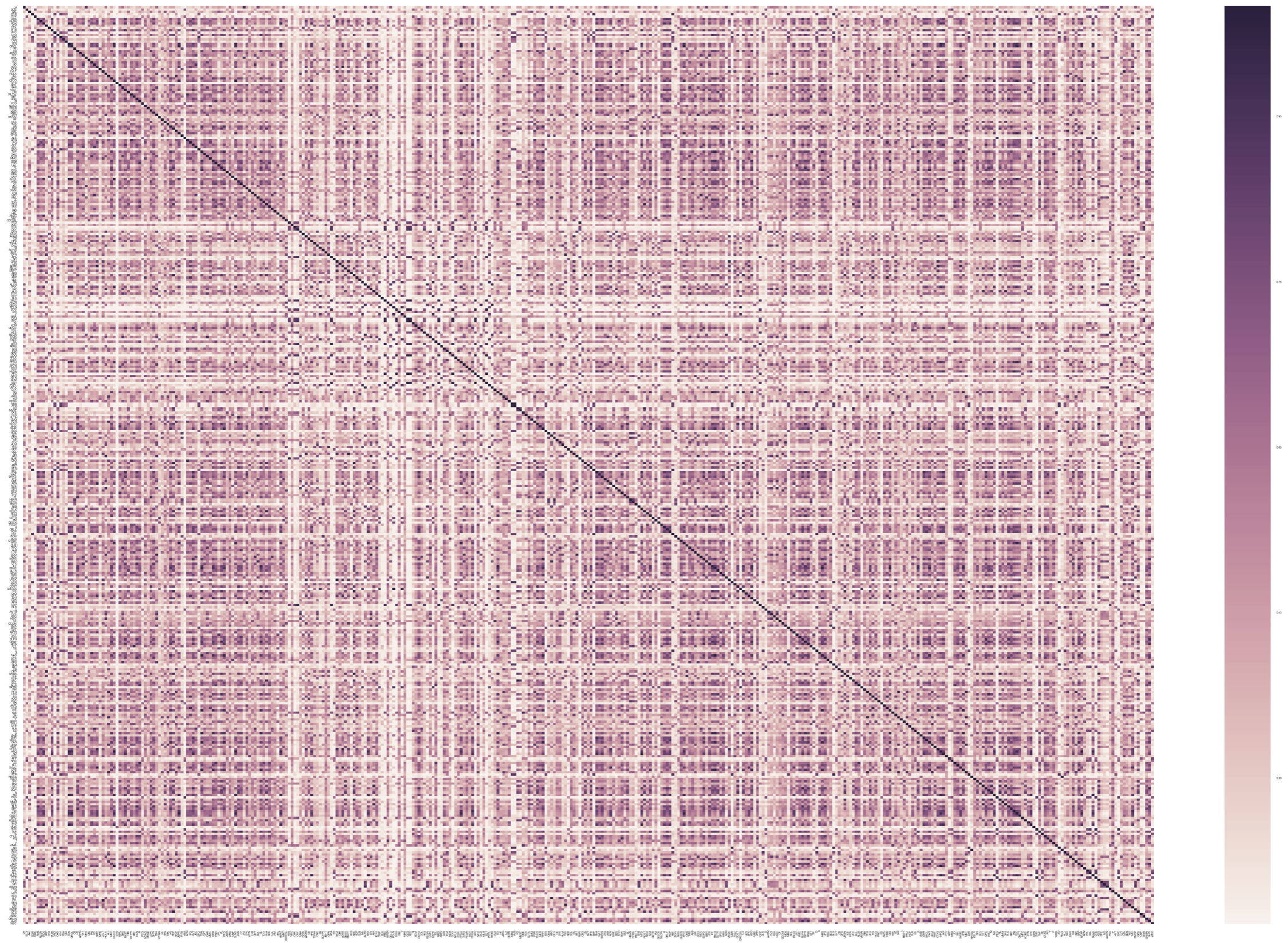
Figure 3 displays the entropy heatmap from LDA topic distributions of all stocks.
Figure 3
Hierarchical Clustering by 10-K Item 1A
Instead of clustering stocks according to business description, it’s also interesting to group them according to risk factors. Doing the same procedure as described before for Item 1A, we obtain the dendrogram displayed in Figure 4.
Figure 4
Topic Modeling of 10-K Item 1A
Observing the topics extracted via SVD in Figure 5, one can identify several topics relating to, e.g., oil, real estate, automotive, and airline risks. Again, the topics are not perfectly clean and hyperparameter tuning and more data will probably improve results considerably.
Figure 5
Conclusion
Use cases for these methods are, for example, statistical arbitrage strategies and portfolio optimization. One can construct very granular clusters of stocks belonging to similar businesses. The similarity matrix can also be input to a function that creates a positive-definite matrix which can then be used as a shrinkage target in covariance matrix estimation.
References
Blei, David M., Andrew Y. Ng, and Michael I. Jordan. “Latent dirichlet allocation.” Journal of machine Learning research 3.Jan (2003): 993-1022.
Portfolio optimization is of central importance to the field of quantitative finance. Under the assumption that returns follow a multivariate normal distribution with known mean and variance, mean-variance optimization, developed by Markowitz (1952), is mathematically the optimal procedure to maximize the risk-adjusted return. However, it has been shown, e.g., by DeMiguel, Garlappi, and Uppal (2007), that out-of-sample performance of optimized portfolios is worse than that of naively constructed ones. The question is why? Do the results break down if the normality assumption is violated? I will show Monte Carlo evidence under heavy tailed distributions that suggest the cause for this strange phenomenon to be a different one.
The actual problem is that, in practice, mean and variance are not known but need to be estimated. Naturally, the sample moments are estimated with some amount of error. Unfortunately, the solution, i.e., the optimal weight vector, to the optimization problem is very sensitive to these estimation errors. The resulting instability of the solution tends to increase with the number of assets in the universe.
To get an intuition why this would happen, imagine uncorrelated assets. Hence, the corresponding (unknown) covariance matrix has only zeros off its diagonal. It is, however, very unlikely that a sample covariance matrix will estimate all off-diagonals to be exactly zero, given a finite sample. You can easily see that the probability that this would happen decreases with . Now, suppose that the estimated sample covariance for some asset and some other asset is some positive number. The optimization algorithm now believes that it can reduce the portfolio risk resulting from longing by shorting . We know, however, that this would not be optimal since the true data generating processes of and are uncorrelated.
The solution to the instability problem is to prevent the optimization algorithm from considering unrelated assets as related. This can be done in two ways. Either we reduce noise in the covariance matrix or we allow hedging between instruments only in certain cases where we have a prior believe that future returns will indeed be correlated. For example, the latter solution implies that we may be comfortable asserting that two airlines expose the portfolio to similar kinds of risk, e.g., oil price, political risk, regulatory risk, travel demand, terror risk, etc., and by selling one of them short we may hedge out these risks resulting from holding long the other. In contrast, just because the sample covariance for an airline stock and some other, totally unrelated, stock is slightly positive, this does not mean we should sell short a large chunk of that second stock to hedge out the risks of the airline stock, although the mean-variance optimizer would regard both scenarios the same.
For me, the best way to get a deeper understanding of the subject is to simulate sample paths, where I know the data generating process, and to observe the behavior of different optimization techniques. In the following, I will compare mean-variance optimization based on sample moments with the same based on a noise-reduced covariance matrix using principal component analysis (PCA). To demonstrate the other approach, I will introduce a hierarchical optimization algorithm, where I use the fact that stocks usually cluster into industries. As a lower bound benchmark, I show results for naive equal weighting. We will see that, out-of-sample, portfolios based on the sample covariance matrix underperform this benchmark substantially. The PCA and hierarchical methods, however, perform significantly better. These results are robust to heavy tailed noise distributions as evidenced by simulated Generalized Autoregressive Conditional Heteroscedasticity (GARCH) sample paths.
But first, let’s simulate a bunch of stocks belonging to different industries. Each stock is composed of a deterministic trend , a loading on the market related stochastic trend and a loading on the industry specific stochastic trend . For each stock, , , and are sampled from a uniform distribution. In the first simulation, I compare mean-variance optimization with a naive diversification approach where each asset is equally weighted with the sign of the expected return. I assume perfect knowledge of the expected return. Traditionally, the expected return is estimated by the in-sample first moment of the asset return. In my example, this would actually make sense since the mean is a consistent estimator of the deterministic trend. In practice, however, there is probably not a stationary deterministic trend. This is where the alpha model steps in, which is not the topic of this study and thus assumed given.
The return of each stock is thus given by
,
where
is the return of asset at time ,
is the th common factor at time ,
is the factor loading or factor beta of asset with respect to factor ,
is the asset-specific factor or asset-specific risk,
,
.
The covariance matrix of the factors, , is . Asset-specific noise is uncorrelated with the factors, i.e., , for , , and . The asset-specific noise is uncorrelated across assets and for each asset it’s serially uncorrelated, i.e.,
.
The diagonal covariance structure reflects the assumption that all correlation between assets is due to the factors.
Let’s write the factor model as
,
where in the matrix ,
,
the th column contains the beta coefficients associated with factor . The covariance matrix of the returns implied by the factor model is
.
Hence, the variance of the returns of asset and the covariance of the returns of asset and are
and
,
respectively. Since the factors are uncorrelated in this simulation, the covariance matrix simplifies to
,
where is the vector of loadings with respect to factor , i.e., the th column of matrix . Thus the variance of asset ‘s returns is
and the covariance between the returns of assets and is
.
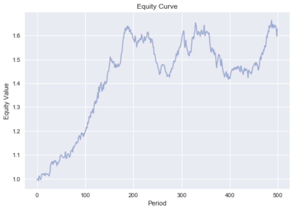
As an example, Figure 1 shows sample paths of 100 stocks belonging to the same industry.
Figure1
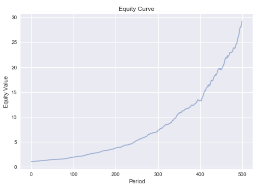
Every stock’s return in this universe is partly driven by the market return (in proportion to its ) and the industry return (in proportion to its ). Hence, one asset can be used to hedge out the factor risks of the other by selling it short. Doing this by mean-variance optimization based on the sample covariance matrix (and known expected return), the resulting portfolio equity under period-wise rebalancing develops as shown in Figure 2.
Figure 2
This very smooth equity curve can be achieved since we can hedge out the systematic factor risk. This makes our bets independent. Independence allows us to reason by the weak law of large numbers that the realized returns will converge in probability to the expected returns. This is only true if short sales are permitted. If we exclude shorting, we can only reduce the asset specific risk while exposing the portfolio to the irreducible systematic risk. The devastating effect this has on our portfolio can be seen by the much more rugged equity curve in Figure 3.
Figure 3
Hierarchical Optimization
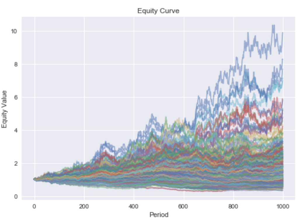
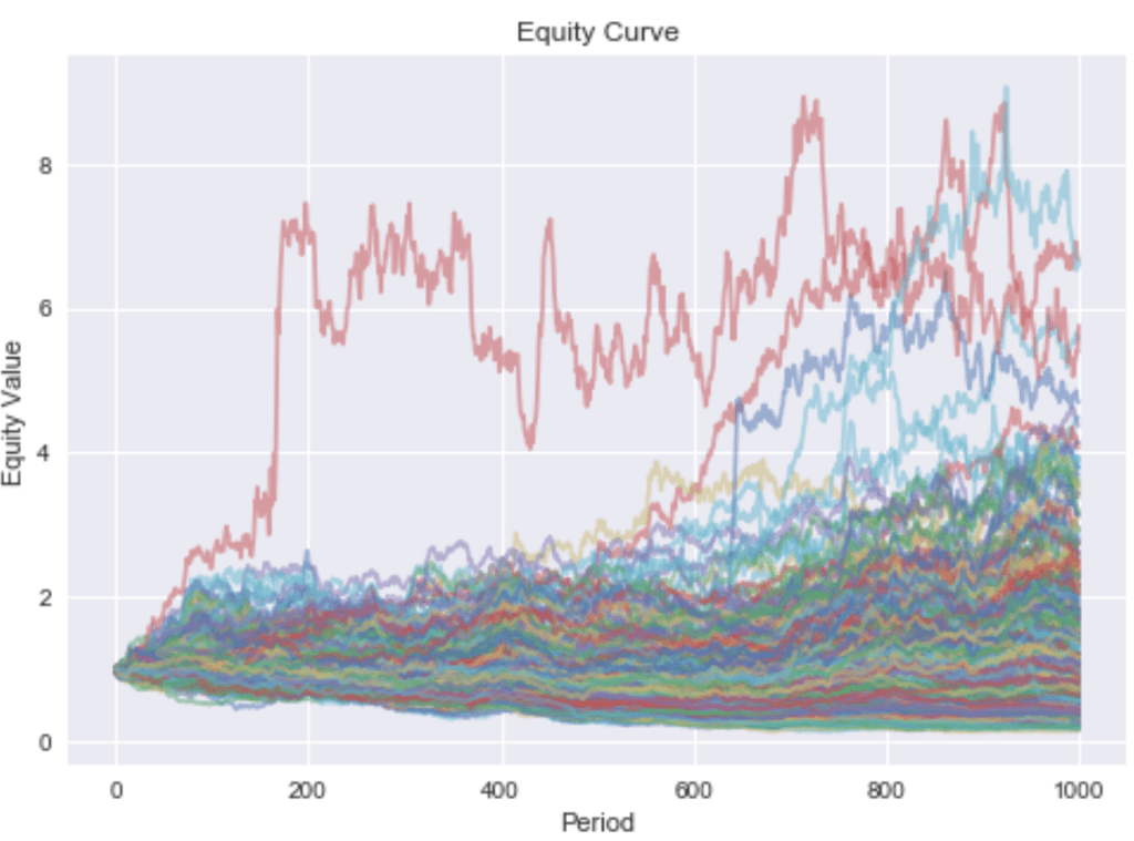
In reality there isn’t just one industry but many. In the following, I will simulate a universe of stocks belonging to nine different industries. The corresponding sample paths are depicted in Figure 4.
Figure 4
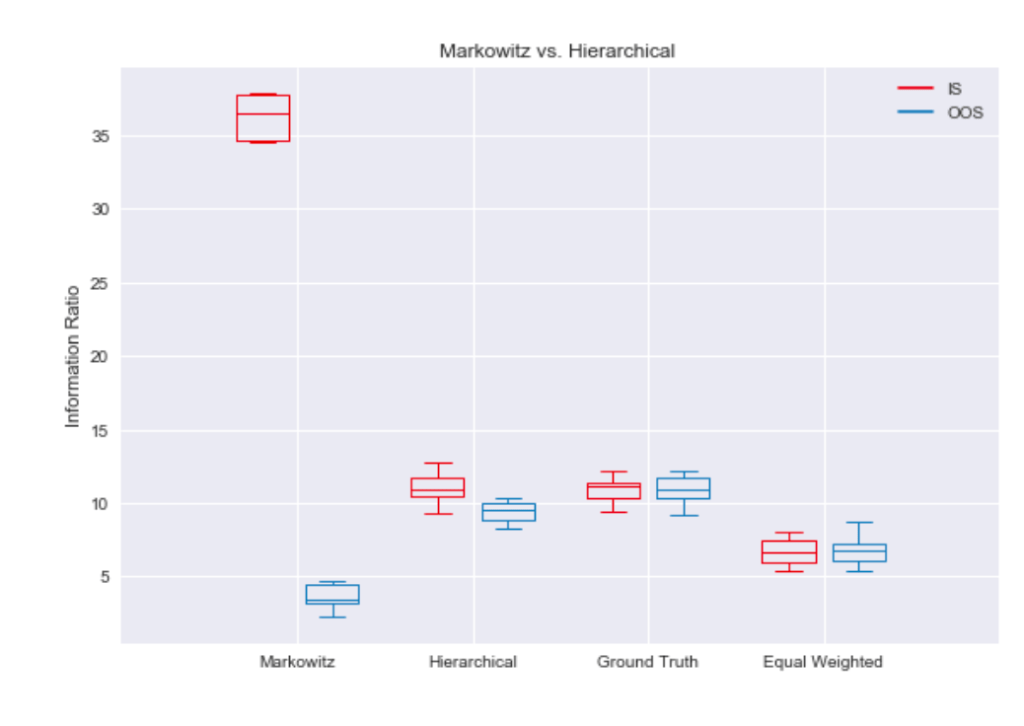
Now, all stocks are still partly driven by the market, but industry returns are uncorrelated. Estimation errors may cause problems if one stock is falsely used as a hedging device for the industry exposure of another stock, and both stocks do not belong to the same industry. The overfit of Markowitz’s method to in-sample data can best be visualized by a boxplot. Figure 5 shows that the in-sample information ratio for the sample covariance optimization is way above the best possible portfolio using ground truth parameters. Unsurprisingly, this overfit hurts the out-of-sample performance, as it can’t even beat simple equal weighting.
Figure 5
If we believe the above characterization of the problem is correct, it seems like a good idea to encode prior knowledge of industry clustering by optimize weights within clusters and then optimize allocation to these clusters. This hierarchical approach results in the in-sample and out-of-sample performance being much closer to the ground truth. Imposing structure, mean-variance optimization now beats equal weighting by a large margin.
Principal Component Analysis
Principal Component Analysis (PCA) allows us to reduce the rank of the covariance matrix. Since the covariance matrix is symmetric positive definite, we can, due to the spectral theorem, decompose the matrix into its real eigenvalues and orthonormal eigenvectors.
with
In the simulation we have exposure to the market and several industries. Thus, it makes sense to reduce the rank to the number of these variables. Plotting the proportion of variance explained by the first principal components in Figure 6 confirms this hypothesis.
Figure 6
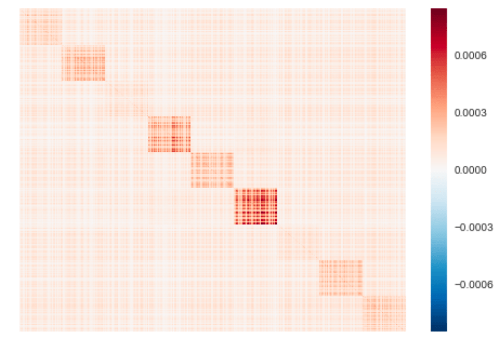
Decomposing the covariance matrix into its eigenvalues and eigenvectors, we can de-noise it by eliminating all eigenvalues below some threshold. Since the sample covariance matrix is positive definite, all its eigenvalues will be positive. Reconstructing a matrix from non-negative eigenvalues will likewise result in a positive semi-definite matrix. We thus don’t have to worry about the resulting matrix not being a proper covariance matrix, which can be a headache with more flexible estimation approaches. A heatmap of the reconstructed covariance matrix from the largest 10 eigenvalues is shown in Figure 7.
Figure 7
This covariance matrix looks very similar to the sample covariance matrix shown in Figure 8, despite having only a rank of 10. We can infer that it captures the important linear relationships between assets with less noise.
Figure 8
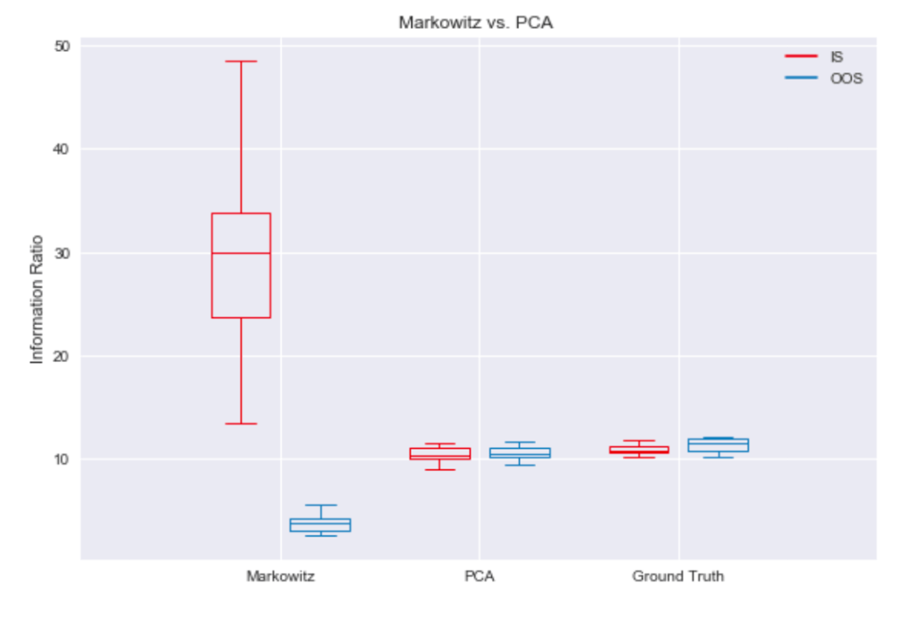
Observing the information ratios depicted in Figure 9, the PCA de-noising method seems capable of restricting factor hedging attempts to reasonable candidates. It beats mean-variance optimization based on the sample covariance matrix in out-of-sample data by a large margin.
Figure 9
Robustness under heavy tailed distributions
Until now, we’ve assumed Gaussian returns. It is a well known fact, though, that real stock return distributions are not Gaussian but heavy tailed. In the following, we will look at simulation results when asset specific noise is modeled by a GARCH process.
Asset specific noise, , is now defined by
,
where
The unconditional variance of asset ‘s specific noise distribution is
,
which, when solved for becomes
.
I use this result to compute the ground truth covariance matrix. Sample paths according to a GARCH(1,1) data generating process are shown in Figure 10.
Figure 10
It’s easy to see that returns are much more extreme than under Gaussian noise. Since Markowitz’s mean-variance optimization tends to over-concentrate and thus expose the portfolio to asset specific risks, which are now heavy tailed, it performs even worse than in the Gaussian case. As shown in Figure 11, the hierarchical method still outperforms equal weighting.
Figure 11
Noise filtering by PCA results in portfolio performances near the ground truth, as can be seen in Figure 12.
Figure 12
Conclusion
To maximize risk-adjusted returns, it is necessary to hedge out systematic risk. How this hedging is done is the subject of portfolio optimization. We’ve seen that it’s important to regularize portfolio optimization, since estimation errors of the covariance matrix would otherwise push out-of-sample performance below that of naive approaches. How to achieve the regularization is a research topic all on its own. We’ve seen two approaches that can be developed far beyond the basics shown here. In addition, correlations between assets tend to be non-stationary. This fact needs to be respected as well. Furthermore, asset returns are driven by multiple factors and business models spread further into sub-clusters within industries. Larger corporations may also belong to multiple clusters. There’s so much more to learn. The code of the simulation, every plot shown here, and all the methods used to compute the portfolio weights is available at https://github.com/jpwoeltjen/OptimizePortfolio.
References
DeMiguel, Victor, Lorenzo Garlappi, and Raman Uppal. “Optimal versus naive diversification: How inefficient is the 1/N portfolio strategy?.” The review of Financial studies 22.5 (2007): 1915-1953.
Markowitz, Harry. “Portfolio selection.” The journal of finance 7.1 (1952): 77-91.
The investing profession is unlike most other professions. To achieve excellent performance you need to act differently than the majority. If a group of proficient engineers collaborate in building a light bulb, they’ll probably come up with a well designed light bulb. This is because there is a solution to this problem that doesn’t depend on other light bulb designs. A light bulb is not a complex adaptive system. In the markets, a similar group of collaboration would not lead to an excellent outcome. Whatever the majority perceives to be right gets priced into the market. It is therefore necessary that actions of the excellent professional are contrary to the opinion of the majority. Of course, this is not yet a sufficient set of conditions. Importantly, the conclusions giving rise to the actions have to be in some kind of way better. I have no doubt the reader realizes that the first element of this argument is contained in the second one, as ‘better’ necessarily implies ‘different’. I think it is useful nonetheless to state the condition explicitly as to not set oneself up for failure. In a strict sense, all the efforts directed to reading books, blogs, news, analyses, and basically anything else by other people would be wasted, not even pointing out the fact that in many cases if they really had this informational edge, why would they sell it to you instead of acting on it themselves gaining much more in the process. I think the argument in its strict form is not always true as e.g. value investing capitalizes on superiority of emotional stamina instead of an informational advantage.
Instead of following well known investing strategies, I’m focussing my efforts on developing systems that generate truly unique strategies. For that it’s useful to state fundamental principles that excellent investing strategies must abide to, and reasoning from there upwards.
Diversification with uncorrelated (or even better negatively correlated) return streams
Compounding
Reducing the risk of catastrophic losses to practically zero
Having an edge
The standard deviation of a portfolio’s return stream declines with the square root of the number of uncorrelated assets (n) within that equally weighted portfolio. It is critically important that these assets — or rather the income streams from trading these assets, which are not the same thing — are uncorrelated. If you had a portfolio of 30 equally weighted assets, and these assets would give you income streams 60% correlated with each other and each stream had a Sharpe ratio — the expected excess rate of return divided by its standard deviation— of 0.2, then the portfolio Sharpe ratio would be: Sharpe_c = n*0.2/(n + 2*n(n − 1)/2 *0.6)^0.5 =0.255. Combining correlated assets only results in a small reduction in risk. Contrast this with the Sharpe ratio assuming uncorrelated assets: Sharpe_u = n*0.2/(n)^0.5 = n^0.5 * 0.2 = 1.095. Here the covariance part of the variance vanishes. The result is a much higher reduction in risk. Furthermore, asymptotically, as n gets large, the risk approaches zero in the uncorrelated case but not in the correlated case. To illustrate, if you would include 100 assets in the portfolio instead of 30, you would get a Sharpe ratio of Sharpe_u = 100^0.5*0.2 = 10*0.2 = 2 in the scenario where the return streams are uncorrelated. Again assuming 60% pairwise correlation, the Sharpe ratio is a mere Sharpe_c = 0.257 for the n=100 portfolio, almost no improvement against the n=30 portfolio.
As I, and this blog, started out with the value investing philosophy, I will shortly run this philosophy by the aforementioned principles. The core principles of value investing match point 2, 3, and 4 — point 1, however, is at odds. Since most value investors are long only stock pickers, diversification is a serious challenge for them. First since a comprehensive fundamental analysis is necessary to evaluate whether or not the investor has an edge in his favor, he will soon reach the limit of his capacity. It is simply not feasible to evaluate thousands of opportunities to come up with a selected basked of, say, 100 stocks without compromising quality. But even if he could, it would not result in true diversification as stocks are correlated and as n gets large the total variance is dominated by the covariance part. This is the reason why many value investors declare diversification beyond a certain threshold — typically between 5 and 50 — as useless and instead focus their funds on their most cherished ideas. If thats not enough to convince you that value investing, as it is practiced by most individuals, has a problem with diversification, consider the fact that Asness et al. (2013) found that the value premium is correlated across asset classes. So even if a more sophisticated value investor would consider a long/short value strategy across even uncorrelated asset classes, the transformation his investment strategy would apply to the asset return streams would yield correlated portfolio constituents. To be clear, I don’t discount value investing as a valuable part of a portfolio. It just can’t be an optimal strategy on its own.
Let’s return to the fundamental principles. The second principle is compounding. As Albert Einstein reportedly said “Compound interest is the eighth wonder of the world. He who understands it, earns it … he who doesn’t … pays it.” Simply put 10% compounded for 100 periods is not 100*10% = 1,000% but 1.1^100-1 = 1,378,000%.
The third principle can be summarized as ‘everything times zero is zero’. It doesn’t matter how stellar one’s track record was, if there is one devastating year, it was all for nought.
The fourth principle is to have an edge. What is meant by this is basically that one has some kind of advantage over one’s competitors such that the expected value of one’s efforts is positive. The easiest —but not the only— way to gain such advantages is to carefully select one’s competitors. The harsh truth about trading the secondary markets is that you have to take the money from someone. It should be arguably more probable to have an edge against less sophisticated investors than against sophisticated professionals. Luckily for the individual trader there are some obvious ways to get out of the way of the most sophisticated professionals. Historically this blog focused on small, obscure stocks that provide opportunities that are not economical for the professional to exploit. Another way is to trade intraday, arguing that there is not enough liquidity in this timeframe for larger funds to employ similar strategies. I’m going to argue that the latter approach is more rewarding as it also allows for more frequent trades and thus more occurrences for the magic of compounding to do its thing.
Where does this rumination lead us? We need a system that generates many uncorrelated trading strategies, ideally trading very often. These strategies then are bundled with proper risk management into a portfolio. To his end I’ve developed a program that takes any data (price, fundamental, sentiment, satellite image data, etc.) and generates a trading strategy for a specified trading frequency. The core of this program is a recurrent neural network (RNN). More specifically, I use Long Short Term Memory (LSTM) units. LSTMs are a specific type of RNN that provide a solution to the vanishing gradient problem as shown by Hochreiter and Schmidhuber (1997). Basically, LSTM cells can look further into the past as traditional RNNs. LSTM networks are one important driver behind the recent advances in machine translation and speech recognition to give only two examples. For more examples read: http://karpathy.github.io/2015/05/21/rnn-effectiveness/.
As a test, I provided the framework only OHLC and datetime information for the EURUSD forex pair. The model extracted a Sharpe ratio of >5 and a CAGR of 60%. I’m the first one to point out that this is not an outcome you should expect to achieve in reality. But the model only gets price data, data that many believe has no predictive power whatsoever. For more information about this project refer to my Github page: https://github.com/jpwoeltjen.
As Warren Buffett rightly says, value and growth are joined at the hip.[1] It seems like a perfectly sensible strategy to pay more for high-quality businesses than for low-quality deep value stocks. And it is… in theory. In practice, it is extraordinarily difficult to find the right trade-off. There has been done some systematic research trying to improve value strategies by including a quality component. Quality, here, means anything one should be willing to pay for (e.g., ROE, ROIC, growth, profitability, etc.) And some of these studies show very counter-intuitive results.
A prominent example of a strategy that supplements a pure value ranking by a quality measure is Joel Greenblatt’s Magic Formula. In their outstanding book “Quantitative Value”, Wesley Gray and Tobias Carlisle show that the quality component actually decreases the performance of a portfolio based on a value ranking alone.[2] The likely reason for this is the mean reverting nature of return on capital, the used quality measure. Economic theory dictates increased competition if companies demonstrate high returns of capital, and exits of competitors if returns are poor. The new competition decreases returns for all suppliers. Exits of competitors increase returns for prevailing businesses. Betting on businesses with historically high returns seems like a bad idea on average, then.
As ambitious bargain hunters, we try to find high-quality businesses at low prices. Studies, however, show that (in competitive markets) valuation is far more important than quality. And in some cases, due to naïve extrapolation of noise traders, quality is actually associated with lower returns. Lakonishok, Shleifer and Vishny (1994) study exactly that. Their results fly in the face of many investors working hard to find the ‘best’ value stocks. Lakonishok et al. construct value portfolios not only based on current valuation ratios but also on past growth. They define the contrarian value portfolio as having a high Book-to-Market ratio (B/M) — the inverse of P/B — and low past sales growth (GS). The reasoning behind this is that by Lakonishok’s et al. definition, value strategies exploit other investor’s negligence to factor reversion to the mean into their forecasts. This is a form of base rate negligence, a tendency in intuitive decision-making found by Kahneman and Tversky (1982).[3] Lakonishok et al. thus identify stocks with low expected future growth (valuation ratio) and low past growth (GS) that indicate naïve extrapolation of poor performance. They show that this definition of value performs better than a simple definition based only on a valuation ratio (e.g., B/M.) Another way of looking at this is by subdividing the high B/M further into high and low past growth. The low past growth stocks outperform the high past growth stocks by 4% p.a. (21.2% vs. 16.8% p.a.) while the B/M ratios of these sub-portfolios “are not very different.” [4]
In his excellent book “Deep Value”, Tobias Carlisle shows insightful statistics for these portfolios. The incredible insight is that even if valuation ratios are practically the same, stocks that rank low on quality (past sales growth) perform better than high-quality stocks. One likely reason is mean reversion in fundamentals.
Similar results are also showing in the deepest of value strategies: net-nets. Oppenheimer (1986) shows that loss-making net-nets outperformed profitable net-nets (36.2% p.a. vs. 33.1%), and non-dividend-paying net-nets outperformed dividend-paying net-nets (40.6% vs. 27.0%) from 1970 to 1983. Carlisle confirms these results out of sample from 1983 to 2010.[5] My own backtests confirm these results from 1999 to 2015. My results at least are, however, mainly driven by the higher discount — profitable businesses don’t usually trade at large discounts to NCAV.
Whether you are a full quant or not, if you are trying to pick the ‘best’ stocks from a value screen you are likely making a systematic mistake — unless you are searching for businesses with moats (i.e., a sustainable competitive advantage that prevents a high return on capital to revert to the mean.) But good luck finding such a business in deep value territory consistently.
Regression to the mean is such a strong tendency and is systematically underestimated by market participants that just betting on historically poorly performing businesses outperforms the market.[6] Bannister (2013) finds that betting on “unexcellent” companies (ranking low on growth, return on capital, profitability) outperformed the market from 1972 to 2013 (13.74% p.a. vs. 10.59%). A portfolio constructed of stocks of “excellent” businesses, in turn, underperformed the market (9.77%).[7]
I still think good quality measures (i.e., measures that do not implicitly bet against regression to the mean in fundamentals) are a potent tool for improving a value ranking. It is, however, not as easy as layering a quality screen blindly over a value screen and thereby imply equal weights. A category of quality measures that is of special interest to me is distress/bankruptcy prediction. But even if the such a measure is very good at identifying value traps, there is still the very serious issue of false positives. That is, excluding stocks that actually perform well on average. A too sensitive measure will likely exclude all the ugliest stocks that perform the best. More research is needed to determine a sensible weighting mechanism. The merit of such a measure is dependent on the false negative error rate, false positive error rate, the cost of false negatives, and, importantly, on the cost of false positives. The cost of false positives may be very high for concentrated portfolios. Even if in studies the quality measure can improve performance, that doesn’t mean that it will improve a concentrated value portfolio (20-30 stocks). The reason is that these studies often hold a very diversified portfolio (e.g., a decile). This is quite a number of stocks. If the quality factor excludes 20 extremely cheap stocks, it’s not a big deal. If you were to hold the 30 cheapest stocks in the universe, however, and the quality factor excludes 20 of them and the next cheapest stocks have 2 times the valuation ratio, it is very likely that the performance will suffer. It will dilute the value factor too much. The important thing is to actually backtest your portfolio and not just rely on studies.
Another interesting area of research lies in identifying moats that prevent mean reversion of high return businesses. That, however, still leaves the question open if these businesses are systematically undervalued.
[3] Kahneman, Daniel and Tverky, Amos: Intuitive Prediction: Biases and Corrective Procedures, in D. Kahneman, P. Slovic, and A. Tversky, Eds.; Judgment Under Uncertainty: Heuristics and Biases, 1982, Cambridge University Press, Cambridge, England.
Many value investors acknowledge that there are many other smart traders, but believe these other traders somehow don’t understand value investing. It appears, a lot of value investors are hugely overconfident when it comes to their special insight, i.e., that value investing works and others just don’t get it. Yet, there is overwhelming evidence that value investing does work and continuous to work even after a lot has been written about it. So, why does the value premium persist? Fortunately, there are better explanations than ignorance. Behavioral finance tries to explain the outperformance of value strategies by differentiating between noise traders, arbitrageurs, and their clients. On the one hand, there has to be someone who, probably due to some bias, e.g. extending the recent negative earnings trend too far into the future and thereby ignoring regression to the mean, sells an asset at a price below fundamental value (the noise trader). On the other hand, there has to be some reason why professional traders with vast resources do not arbitrage this price/value gap away immediately. This is crucial but often ignored. Shleifer and Vishny (1997) explore a possible reason why mispricings may occur even if specialized arbitrageurs are knowledgeable and rational.[1] They do this by assuming that the arbitrageur and the owner of the invested money are two separate entities. According to their model, the arbitrageur’s clients update their prior beliefs about the arbitrageur’s competence by incorporating the recent performance of investments in their assessment. Understanding the limits of arbitrage can help us separating undervalued assets from superficially cheap but not actually underpriced assets.
The key insights are:
In academia, arbitrage is typically defined as riskless without the need of capital. In practice, however, it does require capital (usually part of it from outside investors) and is associated with several forms of risk.
Arbitrage is typically performed by specialized traders who are not well diversified.
Especially in value situations, assets can further decline in price in the short run, even if it is a good bet long-term.
Clients do not have perfect knowledge of the arbitrageur’s competence. It can thus be a rational choice to withdraw capital from an underperforming manager. This forces the manager to sell off assets, even though the expected return actually increased after the price drop.
An agency problem breaks down the link between greater mispricing and higher expected return from the client’s perspective.
This can result in irrational prices while the arbitrageurs and their clients themselves act rationally.
In which situations is arbitrage most limited then?
First and foremost: Small Size. The absolute dollar amount that can be earned arbitraging in extremely small situations is just too small to make the return on invested resources attractive for professional fund managers. This just leaves individual investors. But in the smallest situations, even these investors have to be either inexperienced or so far unsuccessful, or they would have gathered enough capital to make it uneconomical for them as well. Sounds like weak competition to me!
For professional fund managers, very volatile markets increase the risk of looking incompetent in the short term. Therefore, all else equal, we should expect less arbitrage in volatile markets.
The risk of further price declines is greater in situations that take a longer time to play out and are unpredictable. Hence, we should see more arbitrage in strategies that play out (at least partially) before clients can withdraw capital and less when there may be many months or even years of underperformance before the manager is eventually proven right.
Building on that point, this effect should be more severe for assets where there is clearly something wrong — the typical deep value stock. On average, betting on value stocks can be a good idea, but you can look extremely incompetent on any given investment. Hindsight bias compounds this issue. Value situations that do not play out look like stupid investments in hindsight. It might thus be a good idea, as an individual investor, to explicitly focus on situations where one can look extremely incompetent or neglecting on any individual investment to an ignorant outsider (incompetent or self-serving corporate insiders, industry downturn, loss of major customer, negative earnings trend, regulatory issues, etc.)
Of course, identifying areas where mispricings are likely is itself not a viable investment approach. Assets can be undervalued as well as overvalued. But combined with a value ranking, e.g. EV/EBIT, searching in less efficient markets can reduce the risk of buying statistically cheap stocks which prices are actually justified. This is a completely different approach of trying to exclude value traps than the typical qualitative assessment.
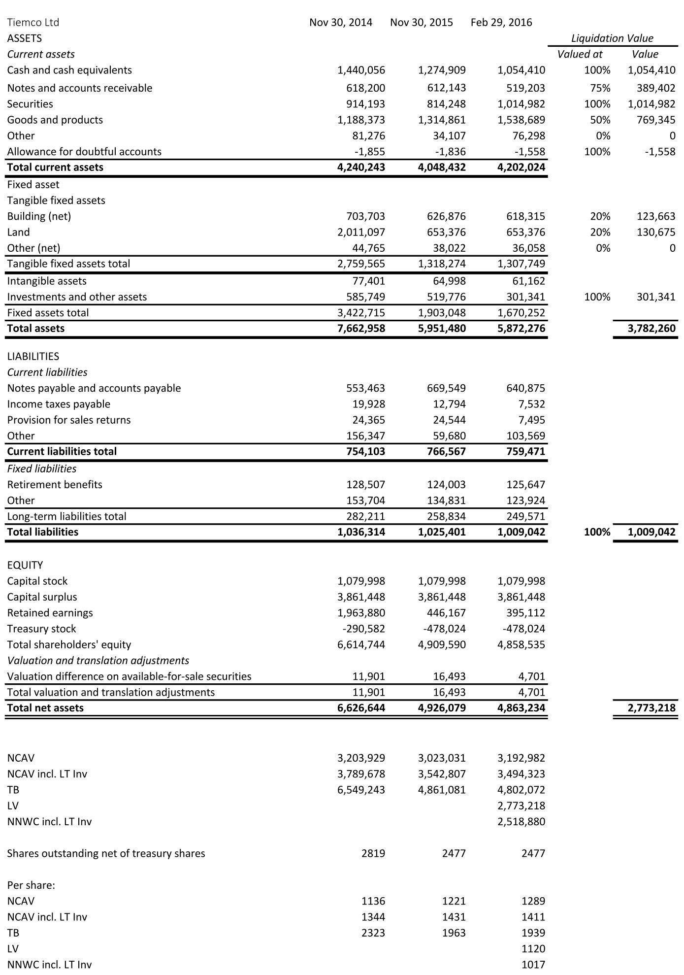
Japanese net-net trading at 34% of NCAV (including LT investments, mostly securities)
The company has recently bought back shares.
Under the radar: Databases (e.g. Bloomberg, Thomson Reuters) have wrong numbers. They do not properly account for treasury shares and thus overstate Tiemco’s market capitalization by 35%. This leads to difficulties in finding this opportunity using stock screeners.
Potentially less sophisticated investor base and limited arbitrage due to very small size. The actual market cap at ¥483/share is ¥1.2 billion ($11 million).
Management expects profitable FY 2016 (ending November, 30). NCAV has been stable over the last years.
Tiemco designs, import, export, and retails fishing goods including lure and fly fishing gears. Tiemco also sells outdoor clothing such as vests, waders, jackets, and goods used for fishing. Source: Bloomberg
Like many other Japanese corporations, Tiemco owns treasury shares. Electronic databases calculate the market capitalization of Japanese corporations using the number of issued shares, not, as would be correct, the number of shares outstanding net of treasury shares. This results in massively upward biased valuation metrics for corporations that own a lot of treasury shares. Therefore, net-nets of that category are hard to find using quantitative stock screeners, which use the numbers supplied by the database. Therein lies the opportunity for mispricings.
Tiemco has recently bought back shares at very cheap prices. As of February 29, 2016, the company owns 863 thousand shares. This is roughly 26% of the 3.340 million total number of issued shares. To illustrate the distortion of valuation metrics that result from using the wrong market cap, consider the discount to NCAV. Using the market cap supplied by the database, one would conclude that Tiemco is trading at a 49% discount to NCAV — interesting, but not quite the 62% actual discount. (Both calculations do not include long-term investments, which are mostly securities, in NCAV.) Assuming the NCAV approximates fair value, the apparent upside of 96% is much less than the actual upside of 163%. Below is the translated balance sheet and the calculation of net current asset value (NCAV), tangible book value (TB), liquidation value (LV), and net-net working capital (NNWC):
Source: Company filings and http://www.kaijinet.com/
Management guides to ¥2.980 billion in sales, ¥49 million in operating income, ¥52 million in ordinary income, and ¥41 million in net income for the fiscal year ending in November 2016.
The Founder and Chairman, Sadahiko Sakai, owns a significant amount of stock. The President, Seiichi Sakai, owns a moderate amount of stock.
Delisting of already hated stock resulted in forced/indiscriminate selling
Stock down over 44% in one day
Balance sheet consists primarily of liquid assets
Insiders own majority of shares
Off the beaten path: Mkt cap = $11.6 million
P/NCAV = 0.24
P/TB = 0.17
P/NNWC = 0.38
On Jan. 22, 2016 QCCO announced plans to delist its stock from the NASDAQ and only provide financial information to stockholders upon request. The following trading day the stock fell off a cliff. QCCO closed at $0.6676 (down 44.38%) while reaching a low of $0.54. I believe the slump is due to indiscriminate selling. While one can make the argument that the stock should trade at a lower valuation because of less liquidity and increased risk. The company will also save money due to lower administrative and legal expenses. At least the drop seems too severe.
“QC Holdings, Inc. Announces Voluntary NASDAQ Delisting and SEC Deregistration
OVERLAND PARK, Kan., Jan. 22, 2016 (GLOBE NEWSWIRE) — QC Holdings, Inc. (NASDAQ:QCCO) announced today that it has notified the NASDAQ Stock Market (“NASDAQ”) of its intention to voluntarily delist its common stock from the NASDAQ Capital Market. The Company intends to cease trading on NASDAQ at the close of business on February 11, 2016. The Company’s obligation to file current and periodic reports with the Securities and Exchange Commission (“SEC”) will be terminated the same day upon the filing of the requisite notification with the SEC. The Company is eligible to deregister its common stock because it has fewer than 300 stockholders of record.
Following delisting and deregistering, the Company presently intends to provide annual information regarding its performance upon stockholder request. The Company’s shares may be quoted in the “Pink Sheets” (www.pinksheets.com), an electronic quotation service for over-the-counter securities. However, there can be no assurance that any market maker or broker will continue to make a market in the Company’s shares.
The Company’s board of directors determined, after careful consideration, that voluntarily delisting and deregistering is in the overall best interests of the Company and its stockholders. Factors that the board of directors considered include the cost savings that will occur as a result of the elimination of the Company’s obligation to file reports with the SEC, the avoidance of additional accounting, audit, legal and other costs and management’s attention devoted to compliance with the requirements of the Sarbanes-Oxley Act of 2002, the historically low daily trading volume in the Company’s shares, and the benefit of allowing management to focus on the long-term development of our core business.”[1]
QC Holdings provides financial services for underbanked customers in 22 States within the USA and in Canada. QCCO advances primarily single-pay loans (payday loans) (~2/3 of revenue) and installment loans through retail branches and their internet lending operations. Payday loans are small short-term loans. The average term of a payday loan is 18 days.[2] The average amount (principal +fee) is $383. Fees represent $59 of that amount so the average fee per $100 advanced is $18 for 18 days![3] This equates to an extremely high annualized interest rate. Many states effectively have banned or have tried to ban payday loans by imposing limits on the annual percentage rate (APR) that can be charged. There were, for example, efforts in Missouri, which accounts for 32% of the gross profit, to place a voter initiative on the statewide ballot for each of the November 2012 and 2014 elections. The voter initiative was intended to place a limit APR of 36% on any lending in the state. There weren’t enough valid signatures, however, to place the initiative on the ballot of either of the elections. Such a limit would render the provision of payday loans unprofitable.
The amount advanced under installment loans ranges from $400 to $3000.
QCCO offers branch-based installment loans to customers in eight states. Branch-based installment loans are very similar to payday loans in principal amount, fees and interest, but allow the customer to repay the loan in bi-weekly installments. In 2014, branch-based installment loans were offered in 194 locations and accounted for 13.7% of total revenues.
During 2014, the average principal amount of a signature loan was $1,845 and the average term was 20 months. In 2014, signature loans accounted for 10.6% of revenue and were offered in over 200 locations in Arizona, California, Idaho, Missouri, New Mexico and Utah.
Auto equity loans are higher-dollar installment loans secured by the borrower’s auto title with a typical term of 12 to 48 months and a principal balance of up to $15,000. Fees and interest vary based on the size and term of the loan. During 2014, the average principal amount of an auto equity loan was $3,421 and the average term was 32 months. As of December 31, 2014, QCCO offered auto equity loans to customers at 134 branches in Arizona, California, Idaho, New Mexico and Utah.[4] In February 2015, the Company completed the sale of its auto facility for approximately $1.2 million, net of fees to an unrelated third party. The net book value of the property sold was approximately $1.2 million.[5]
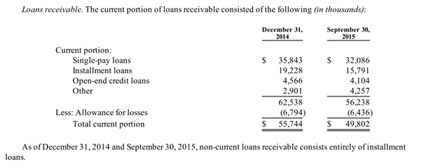
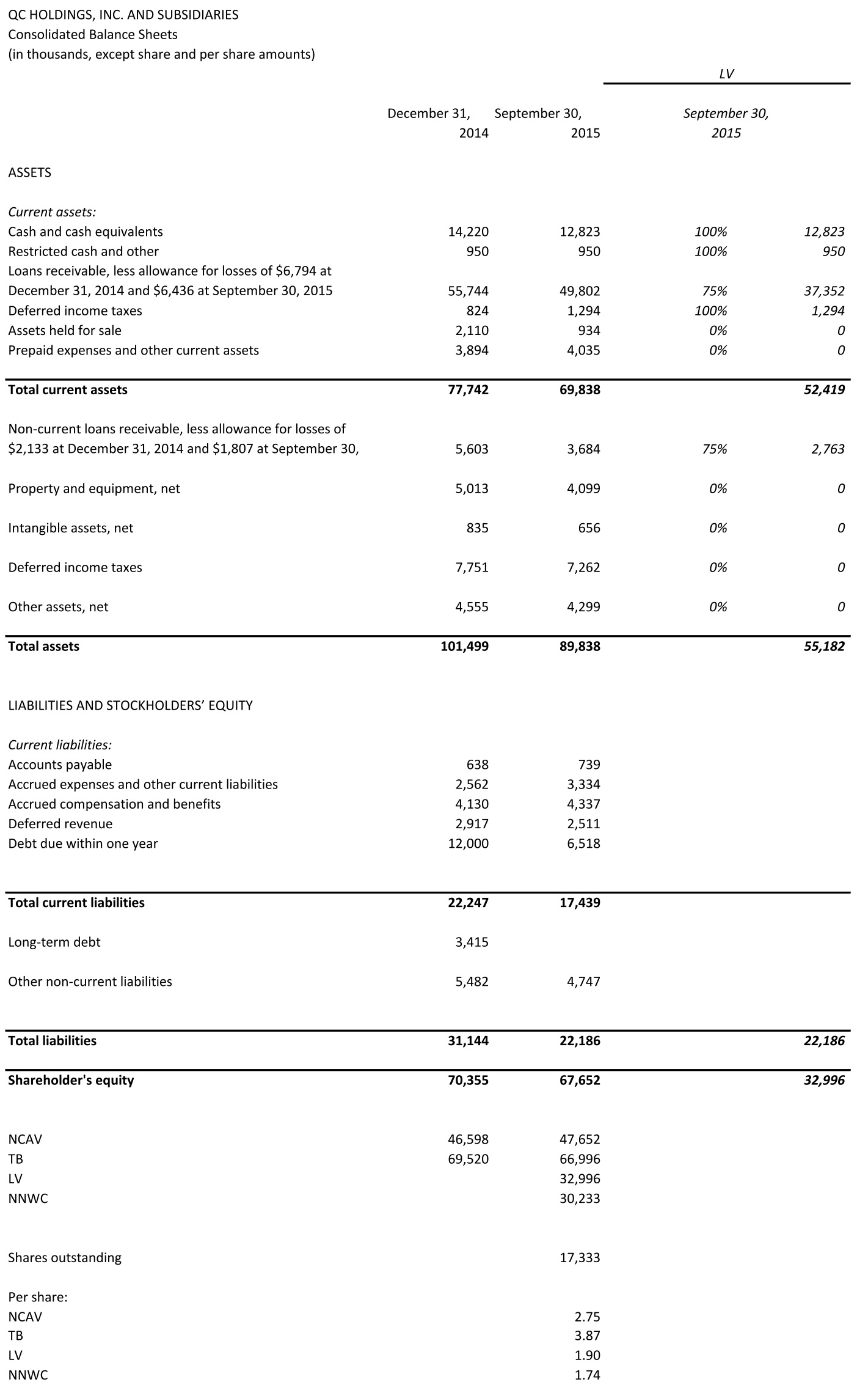
The balance sheet consists primarily of cash and short-term loans receivable. How much are the loans receivable worth? I think close to book value. To be conservative, however, I cut off 25% for my liquidating value.
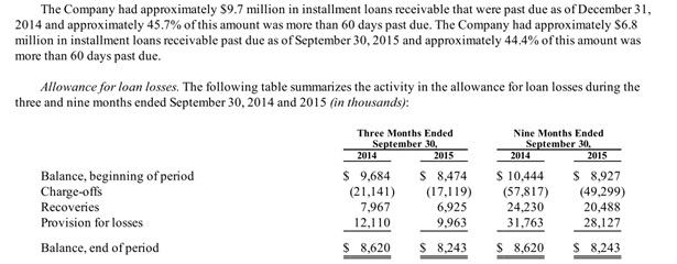
“The overall provision for payday loan losses during 2014 was approximately 2.8% of total payday loan volume (including Internet lending). On average, the overall provision for payday loan losses has historically ranged from 2% to 5% of total payday loan volume.”[6]
Below are the calculations of net current asset value (NCAV), tangible book value (TB), liquidating value (LV) and net-net working capital (NNWC).
Source: 10-Q 09/2015
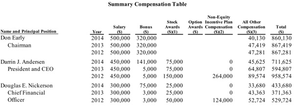
There are some things I really don’t like about this company. First, I am very skeptical about the viability of the business. Customers explore alternatives and many states want to effectively ban the services QCCO provides. Yet, management stated their intention to expand the business. Second, the compensation of management is high. There is also a loan from the chairman to the company at a 16% interest rate.
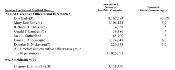
On the other hand, management owns the majority of the stock outstanding. Owning over 8 million shares the chairman should be incentivized to act in the shareholder’s best interest — even after considering the high compensation.
I have no opinion where the stock will trade in the short-term. It can certainly become much cheaper. Dark companies can trade at extreme discounts. I think, however, the stock is a good statistical bet at this price. I like the high liquidity of QCCO’s assets and the alignment of the shareholder’s and chairman’s interest due to his substantial stock holding.
Disclosure: I currently have no position in QCCO but intent to initiate a long position in the next days.
62 % discount to NCAV + net long-term investment securities and deposits
69% discount to tangible book value
Negative enterprise value
Management guides to a profitable FY
US$12.7 million market cap
Reporting in Japanese, only
Holding ~15% of own shares in treasury
Solekia Ltd. engages in the IT-related business. It operates through the following segments: Tokyo Metropolitan Area, Eastern Japan, Western Japan, and Others. Solekia sells electronic devices, electronic wires and cables, wire related products, data processing system and software, and telecommunication equipment. The Company also designs, develops, and provides consultation for semiconductors, information and communication systems, and multimedia systems. The company was founded in 1958 and is headquartered in Tokyo, Japan.
The company is currently profitable and management expects the second half and the full FY ending March 31, 2016 to be profitable, as well:
Guidance for fiscal year ending March 31, 2016:
Sales: ¥21.300 million
Operating income: ¥170 million
Ordinary income: ¥195 million
Net income: ¥70 million
Net income per share: ¥80.58
Solekia is tiny. Its market cap is ¥1,526 million (= $12.691 million). Only reporting in Japanese, the stock is under the radar for a substantial part of the investing community. The company owns roughly 15% of its issued shares. Many databases provide inaccurate information for Solekia. Together this makes the stock truly off-the-beaten-track.
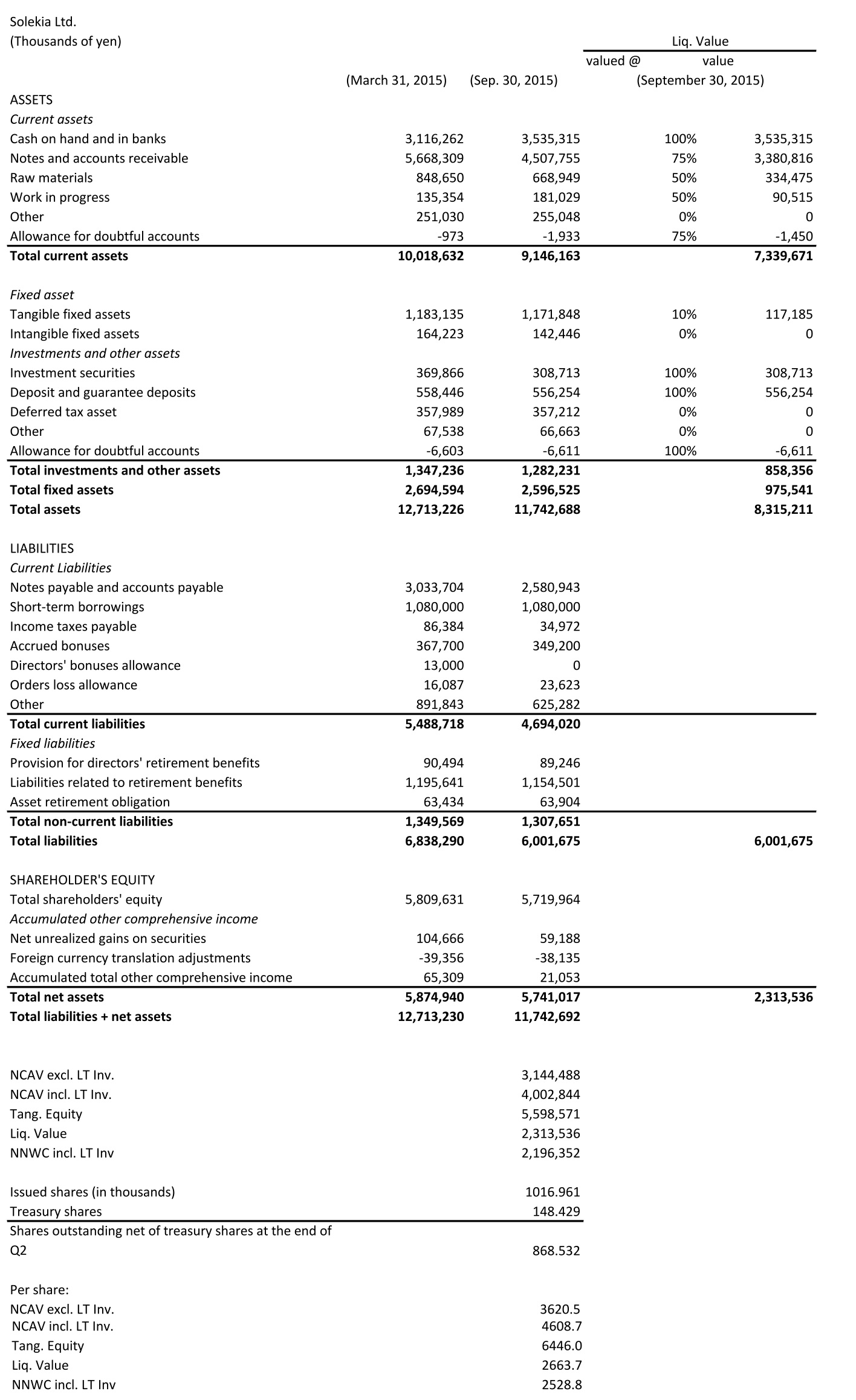
Solekia trades at a 51% discount to NCAV. If one includes net long-term investment securities and deposits, the discount increases to 62%. I found nothing that would qualify as a hard catalyst. I also couldn’t find signs of off-balance-sheet liabilities, contingent liabilities or significant litigation. The thesis is plain mean reversion.
Below is the translated balance sheet using Google Translate, the approximation of liquidation value and the calculations of net current asset value, net-net working capital and tangible book value.
(Source: Quarterly Report for the Second Quarter Ending September 30, 2015 Translated via Google Translate)
The President owns a small amount of shares.
Disclosure: I currently have no position in 9867:Tokyo.
I cannot read Japanese and rely on Google Translate to read the documents. I might miss something important.
Market capitalization: ¥2,743 million (US$22.37 million)
P / t. B = 0.28
P / NCAV = 0.38
P / Liq. value = 0.56
P / NNWC = 0.61
Katsuragawa Electric manufactures large format printers, copiers and micro motors. This obviously isn’t exactly a growth industry. I expect the printer business, in general, to slowly decline in the future. I think, however, at these prices, the stock is trading significantly below intrinsic value. At ¥179, the stock is trading at a 62% discount to NCAV (including net long-term investments). The company is currently marginally unprofitable. Management guides to a profitable FY 2016 (ending March 2016), however. They expect ¥110 million in ordinary income, from which ¥10 million is attributable to holders of the parent, ¥140 million in operating income and ¥10,500 million in sales for FY 2016. Management identifies the usual suspects to restore profitability: streamlining, reducing fixed costs, better inventory management, cutting executive compensation, firing people and developing new sources of revenue – nothing extraordinary that qualifies as a hard catalyst. On the other hand, I also couldn’t find (which doesn’t mean there aren’t) any signs of major adverse litigation, off-balance-sheet-liabilities etc. that might indicate severely negative surprises in the future. Below is the translated balance sheet, calculation of NCAV, NNWC and a conservative approximation of liquidation value:
(Source: Quarterly Reports for the First and Second Quarter Ending June 30, 2015 and September 30, 2015 Translated via Google Translate)
I want to reemphasize that I can’t read a word in Japanese and might miss something important. This stock represents only a small position in my diversified net-net basket. Decisions in this basket are based almost entirely on quantitative variables.


 uncorrelated assets. Hence, the corresponding (unknown) covariance matrix has only zeros off its diagonal. It is, however, very unlikely that a sample covariance matrix will estimate all off-diagonals to be exactly zero, given a finite sample. You can easily see that the probability that this would happen decreases with
  and some other asset
  is some positive number. The optimization algorithm now believes that it can reduce the portfolio risk resulting from longing
  , a loading on the market related stochastic trend
  and a loading on the industry specific stochastic trend
  . For each stock,
  ,
,  is the return of asset
  ,
,  is the
  th common factor at time
  is the factor loading or factor beta of asset
  is the asset-specific factor or asset-specific risk,
  ,
, .
.  covariance matrix of the factors,
 ![\boldsymbol{f}_{t}=\left[f_{1 t}, f_{2 t}, \ldots, f_{k t}\right]^{\prime}](https://s0.wp.com/latex.php?latex=%5Cboldsymbol%7Bf%7D_%7Bt%7D%3D%5Cleft%5Bf_%7B1+t%7D%2C+f_%7B2+t%7D%2C+%5Cldots%2C+f_%7Bk+t%7D%5Cright%5D%5E%7B%5Cprime%7D&bg=ffffff&fg=303030&s=0&c=20201002) , is
, is  . Asset-specific noise is uncorrelated with the factors, i.e.,
  , for
, for  . The asset-specific noise is uncorrelated across assets and for each asset it’s serially uncorrelated, i.e.,
![{\qquad \boldsymbol{\Sigma}_{\boldsymbol{\epsilon}}=\mathrm{Cov}\left(\boldsymbol{\epsilon}_{t}\right)=\left[\begin{array}{cccc}{\sigma_{\epsilon_{1}}^{2}} & {0} & {\cdots} & {0} \\ {0} & {\sigma_{\epsilon_{2}}^{2}} & {\cdots} & {0} \\ {\vdots} & {\vdots} & {\ddots} & {\vdots} \\ {0} & {0} & {\cdots} & {\sigma_{\epsilon_{N}}^{2}}\end{array}\right]}](https://s0.wp.com/latex.php?latex=%7B%5Cqquad+%5Cboldsymbol%7B%5CSigma%7D_%7B%5Cboldsymbol%7B%5Cepsilon%7D%7D%3D%5Cmathrm%7BCov%7D%5Cleft%28%5Cboldsymbol%7B%5Cepsilon%7D_%7Bt%7D%5Cright%29%3D%5Cleft%5B%5Cbegin%7Barray%7D%7Bcccc%7D%7B%5Csigma_%7B%5Cepsilon_%7B1%7D%7D%5E%7B2%7D%7D+%26+%7B0%7D+%26+%7B%5Ccdots%7D+%26+%7B0%7D+%5C%5C+%7B0%7D+%26+%7B%5Csigma_%7B%5Cepsilon_%7B2%7D%7D%5E%7B2%7D%7D+%26+%7B%5Ccdots%7D+%26+%7B0%7D+%5C%5C+%7B%5Cvdots%7D+%26+%7B%5Cvdots%7D+%26+%7B%5Cddots%7D+%26+%7B%5Cvdots%7D+%5C%5C+%7B0%7D+%26+%7B0%7D+%26+%7B%5Ccdots%7D+%26+%7B%5Csigma_%7B%5Cepsilon_%7BN%7D%7D%5E%7B2%7D%7D%5Cend%7Barray%7D%5Cright%5D%7D&bg=ffffff&fg=303030&s=0&c=20201002) .
. ,
, matrix
  ,
, ![{\qquad \boldsymbol{B}=\left[\begin{array}{c}{\boldsymbol{\beta}_{1}^{\prime}} \\ {\boldsymbol{\beta}_{2}^{\prime}} \\ {\vdots} \\ {\boldsymbol{\beta}_{N}^{\prime}}\end{array}\right]=\left[\begin{array}{cccc}{\beta_{11}} & {\beta_{12}} & {\cdots} & {\beta_{1 k}} \\ {\beta_{21}} & {\beta_{22}} & {\cdots} & {\beta_{2 k}} \\ {\vdots} & {\vdots} & {\ddots} & {\vdots} \\ {\beta_{N 1}} & {\beta_{N 2}} & {\cdots} & {\beta_{N k}}\end{array}\right]}](https://s0.wp.com/latex.php?latex=%7B%5Cqquad+%5Cboldsymbol%7BB%7D%3D%5Cleft%5B%5Cbegin%7Barray%7D%7Bc%7D%7B%5Cboldsymbol%7B%5Cbeta%7D_%7B1%7D%5E%7B%5Cprime%7D%7D+%5C%5C+%7B%5Cboldsymbol%7B%5Cbeta%7D_%7B2%7D%5E%7B%5Cprime%7D%7D+%5C%5C+%7B%5Cvdots%7D+%5C%5C+%7B%5Cboldsymbol%7B%5Cbeta%7D_%7BN%7D%5E%7B%5Cprime%7D%7D%5Cend%7Barray%7D%5Cright%5D%3D%5Cleft%5B%5Cbegin%7Barray%7D%7Bcccc%7D%7B%5Cbeta_%7B11%7D%7D+%26+%7B%5Cbeta_%7B12%7D%7D+%26+%7B%5Ccdots%7D+%26+%7B%5Cbeta_%7B1+k%7D%7D+%5C%5C+%7B%5Cbeta_%7B21%7D%7D+%26+%7B%5Cbeta_%7B22%7D%7D+%26+%7B%5Ccdots%7D+%26+%7B%5Cbeta_%7B2+k%7D%7D+%5C%5C+%7B%5Cvdots%7D+%26+%7B%5Cvdots%7D+%26+%7B%5Cddots%7D+%26+%7B%5Cvdots%7D+%5C%5C+%7B%5Cbeta_%7BN+1%7D%7D+%26+%7B%5Cbeta_%7BN+2%7D%7D+%26+%7B%5Ccdots%7D+%26+%7B%5Cbeta_%7BN+k%7D%7D%5Cend%7Barray%7D%5Cright%5D%7D&bg=ffffff&fg=303030&s=0&c=20201002) ,
,![\boldsymbol{R}_{t}=\left[R_{1 t}, R_{2 t}, \ldots, R_{N t}\right]](https://s0.wp.com/latex.php?latex=%5Cboldsymbol%7BR%7D_%7Bt%7D%3D%5Cleft%5BR_%7B1+t%7D%2C+R_%7B2+t%7D%2C+%5Cldots%2C+R_%7BN+t%7D%5Cright%5D&bg=ffffff&fg=303030&s=0&c=20201002) implied by the factor model is
implied by the factor model is  .
.
 ,
, ,
, is the vector of loadings with respect to factor
 .
.

 with
with 
 principal components in Figure 6 confirms this hypothesis.


 , is now defined by
  ,
,


 ,
, becomes
 .
.

 Source: Company filings and http://www.kaijinet.com/
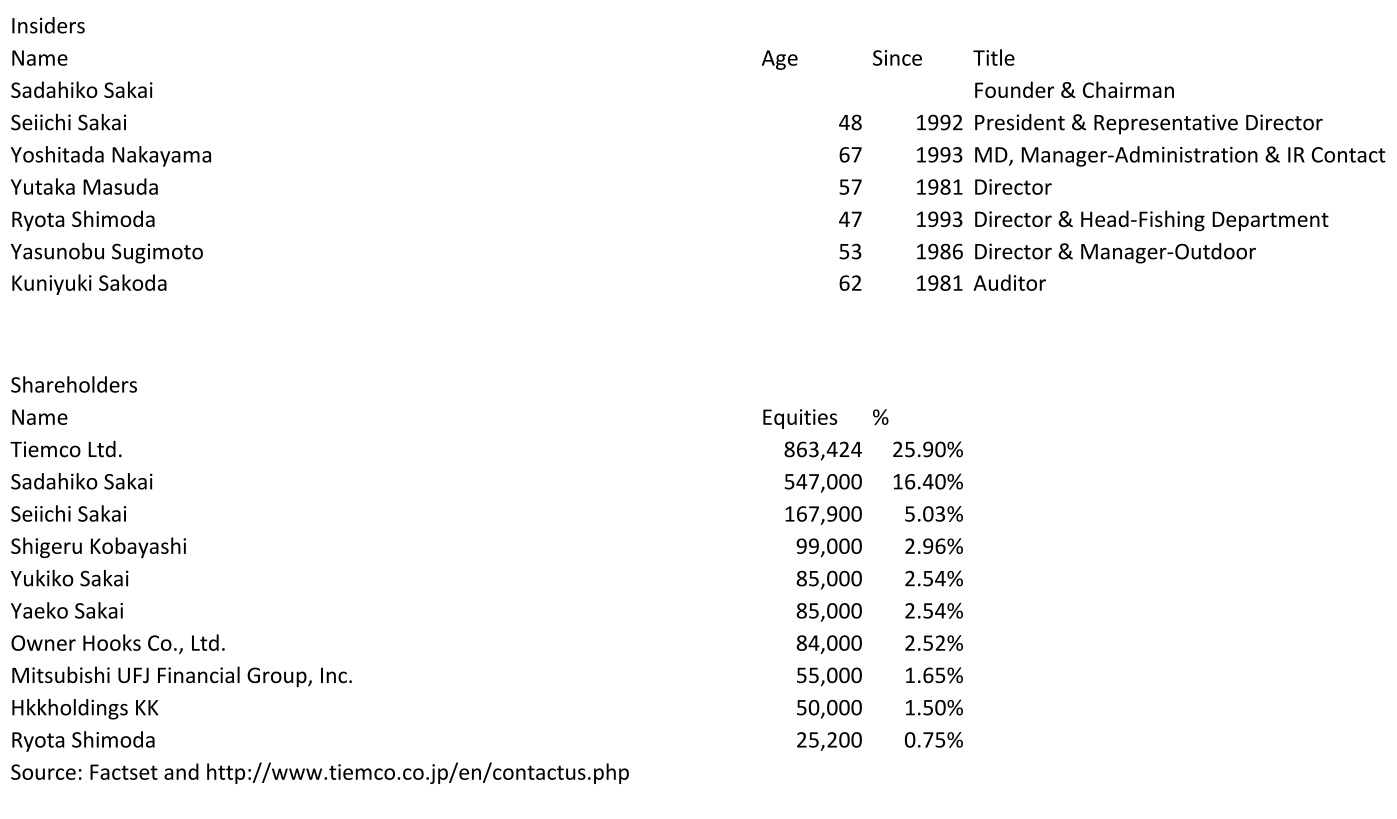


 (Source: Quarterly Report for the Second Quarter Ending September 30, 2015 Translated via Google Translate)